DIP_review_2_2
DIP_review_2_2 - Image reconstruction & Restoration
1. Noise
- 噪声一般可以用PDF表示,因此我们可以进行参数估计
- ,
1.1 Periodic Noise
- sinusoidal noise(在频率域中以共轭冲激串的形式出现)
- cosine noise
- 适合用频率域滤波器解决,如Bandpass filter & Notch filter
1.2 Random Noise
-
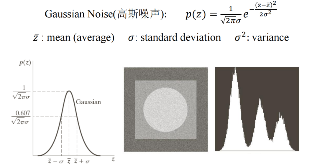
- Gaussian noise
-
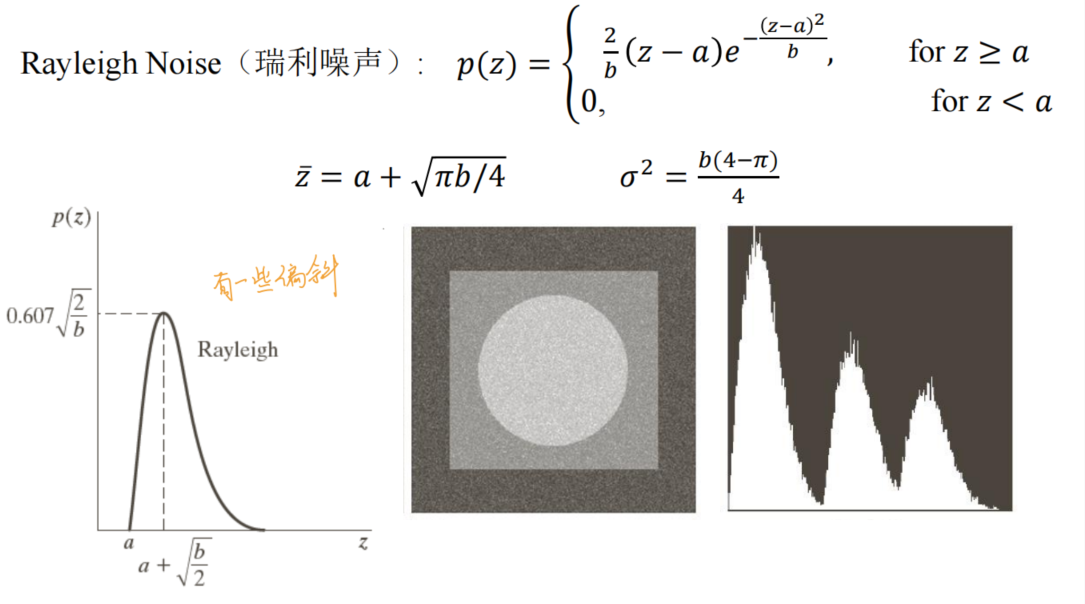
- Rayleigh noise
-
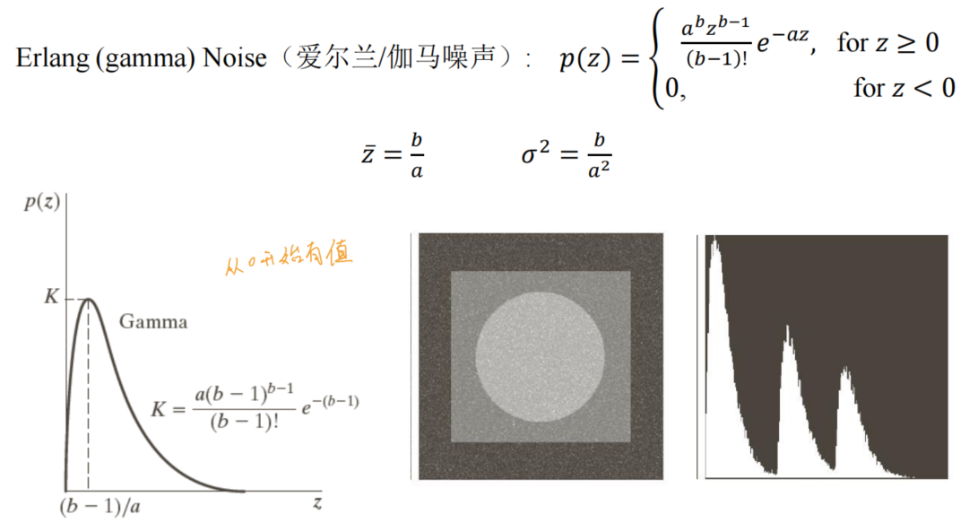
- Gamma noise
-
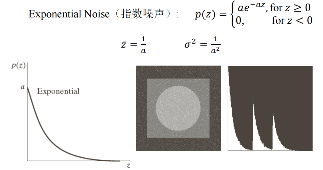
- Exponent noise
-
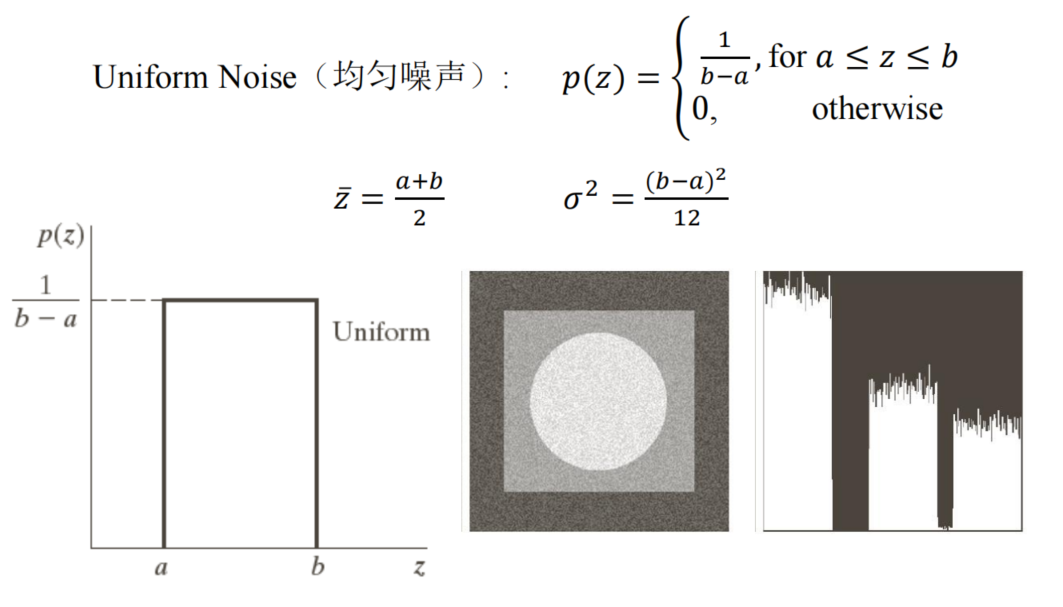
- Uniform noise
-
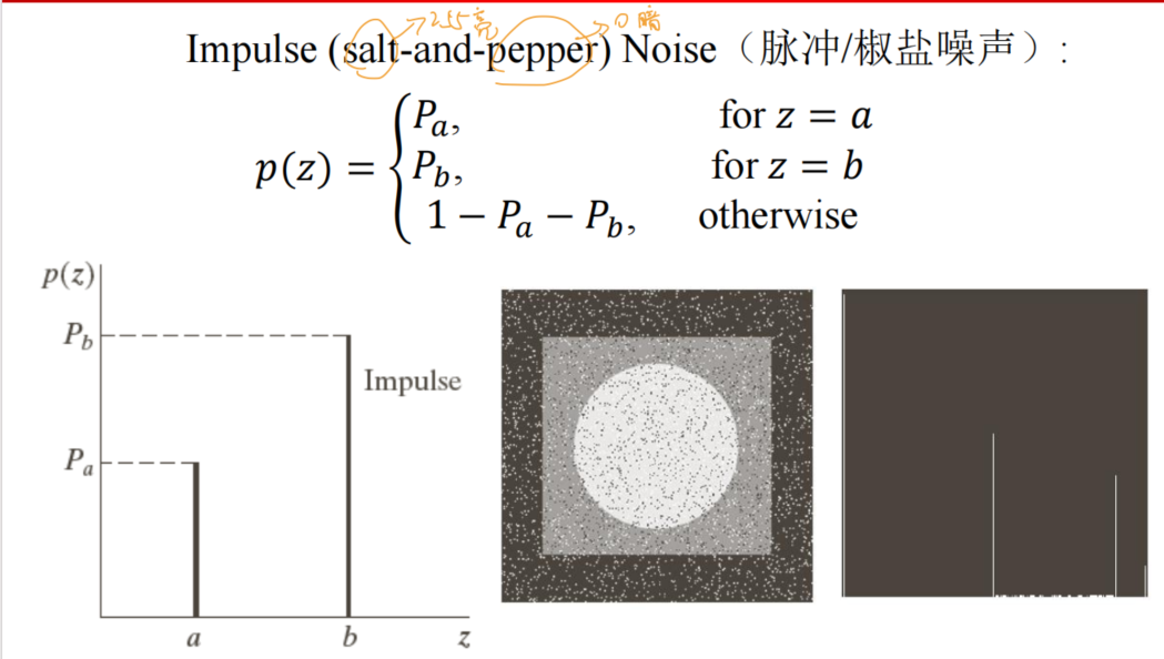
- Salt and pepper noise
- 适合用空间滤波器进行滤波
-
- 噪声与空间坐标无关
-
- 噪声之间相互独立
-
- 噪声与图片像素无关
-
2. Filter(这一部分与review 1部分有所重合)
2.1 Spatial filter
2.1.1 Mean Filters
- Arithmetic mean filter
- Geometric mean filter
- 适用于解决高斯/均匀噪声
- Harmonic mean filter(谐波均值滤波器)
- Contraharmonic mean filter(逆谐波均值滤波器)
- 当, 此时的逆谐波均值滤波器等于谐波均值滤波器
- 当, 适用于处理pepper noise即黑噪声
- 当, 适用于处理salt noise即白噪声
2.1.2 Order-statistic Filters
- Median filter
- 适用于处理比例不太大,的salt and pepper noise
- Max filter
- 适用于处理pepper noise
- Min filter
- 适用于处理salt noise
- Midpoint filter
- Alpha-trimmed mean filter
- 本质是舍弃patch中前后各,因此适用于处理椒盐噪声
2.1.3 Adaptive Filters(具有更强的细节保留能力,如edge)
- Adaptive Median filter(自适应中值滤波器)
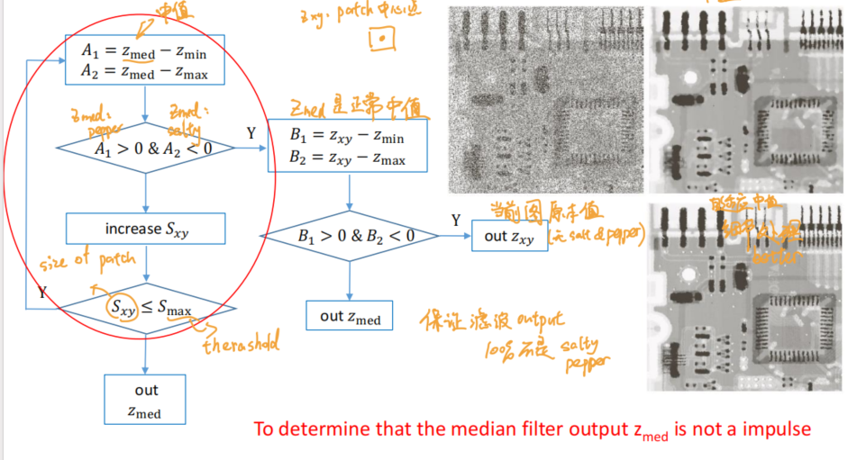
- 第一部分为寻找合适的patch以及对应的。当找到合适的在该patch中,那么进入第二部分。否则扩大patch的size直至阈值去寻找。若大于阈值时仍未找到,说明该部分无法improve,输出等于最大值或是最小值的
- 第二部分为寻找某一点的最好输出。若该点的original pixel value就处于正常范围内则直接输出,否则输出
- Adaptive, Local Noise-reduction filter 局部噪声抑制滤波器
- Suppose we already know
- 退化图像
- 整个图像的噪声方差
- 局部均值
- 局部方差
- Principle:
- If , then . 说明噪声方差在全图为0,直接等于原图即可
- If $ \frac{\sigma_y^2}{\hat{\sigma}_L^2} \approx 1$, then . 说明局部的方差与噪声相似,用均值替换来消除噪声
- If , then . 说明局部的方差大,特征更重要,比如edge,因此需要保留局部特征
- Suppose we already know
2.2 Frequency filter(This part has also been discussed in previous review)
2.2.1 Optimum Notch Filters 最佳陷波滤波器
- step 1: Notch pass filter 扣出噪声
- step 2: 再减去噪声*最优系数
- step 3: 估计local方差
- step 4: 最小化方差,找到最优系数
3. Model of Image Degradation 图像退化模型
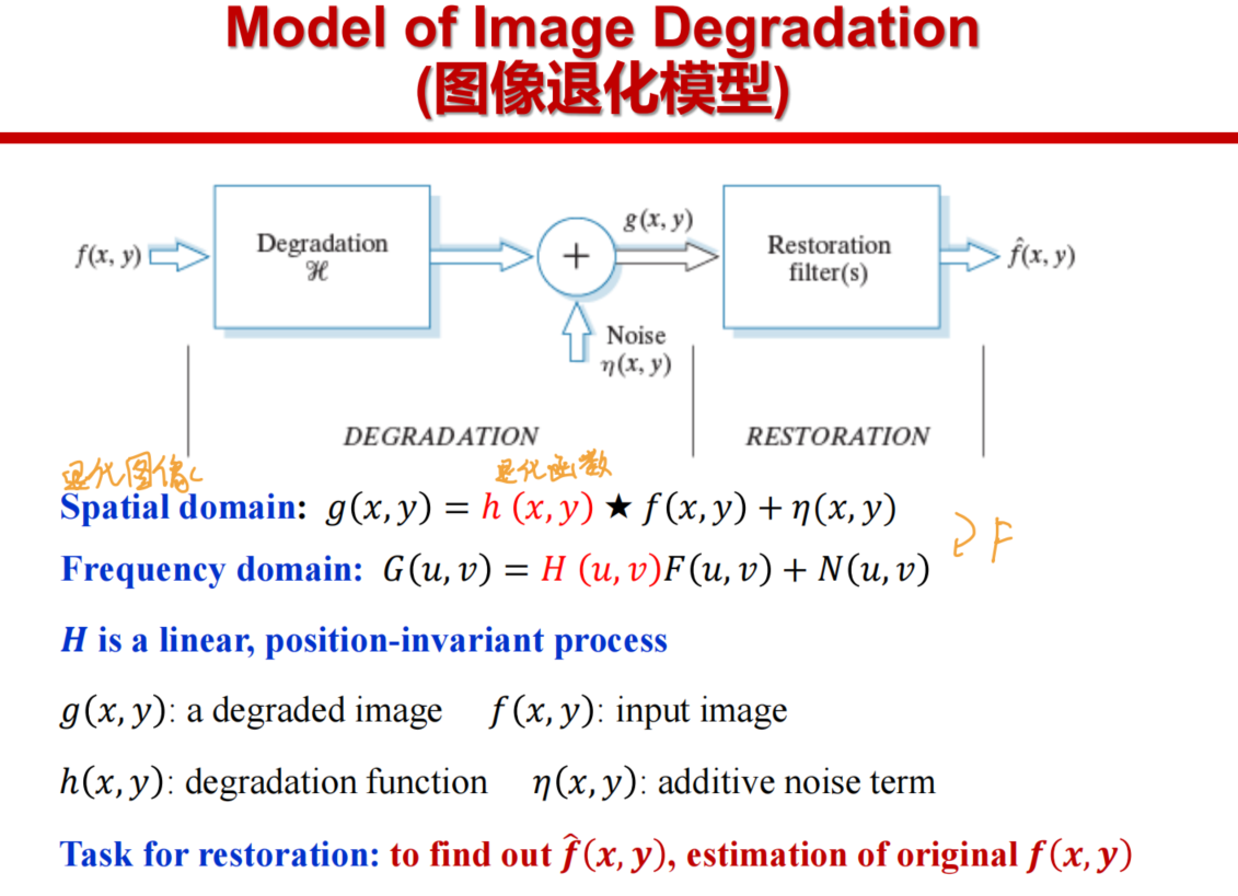
- Model Assumption
- Linear, position-invariant degradation system
- Estimate the degradation function (求 )
- Estimation by Image observation
- , G known and F estimate
- Estimation by experimentation
- , A strength of the impulse response
- Estimation by modeling
- Estimation by Image observation
- Image restoration (求 )
- Inverse filtering
- Problem: 当H太小时,会导致噪声在该点的意外放大,影响该点restore的效果
- Sol: limit the frequency around the origin
- Wiener filtering 维纳滤波
- Goal:
- $\hat{F}(u,v)=[\frac{H^{*}(u,v)}{|H(u,v)|^2 + \frac{S_n(u,v)}{S_f(u,v)}}]G(u,v) = [\frac{1}{H(u,v)}\frac{|H(u,v)|^2}{|H(u,v)|^2 + \frac{S_n(u,v)}{S_f(u,v)}}]G(u,v) $
- , , 信噪比的倒数,若无噪声则退化为Inverse Filtering
- 由于未知,退化为,来对
K进行调参
- Inverse filtering
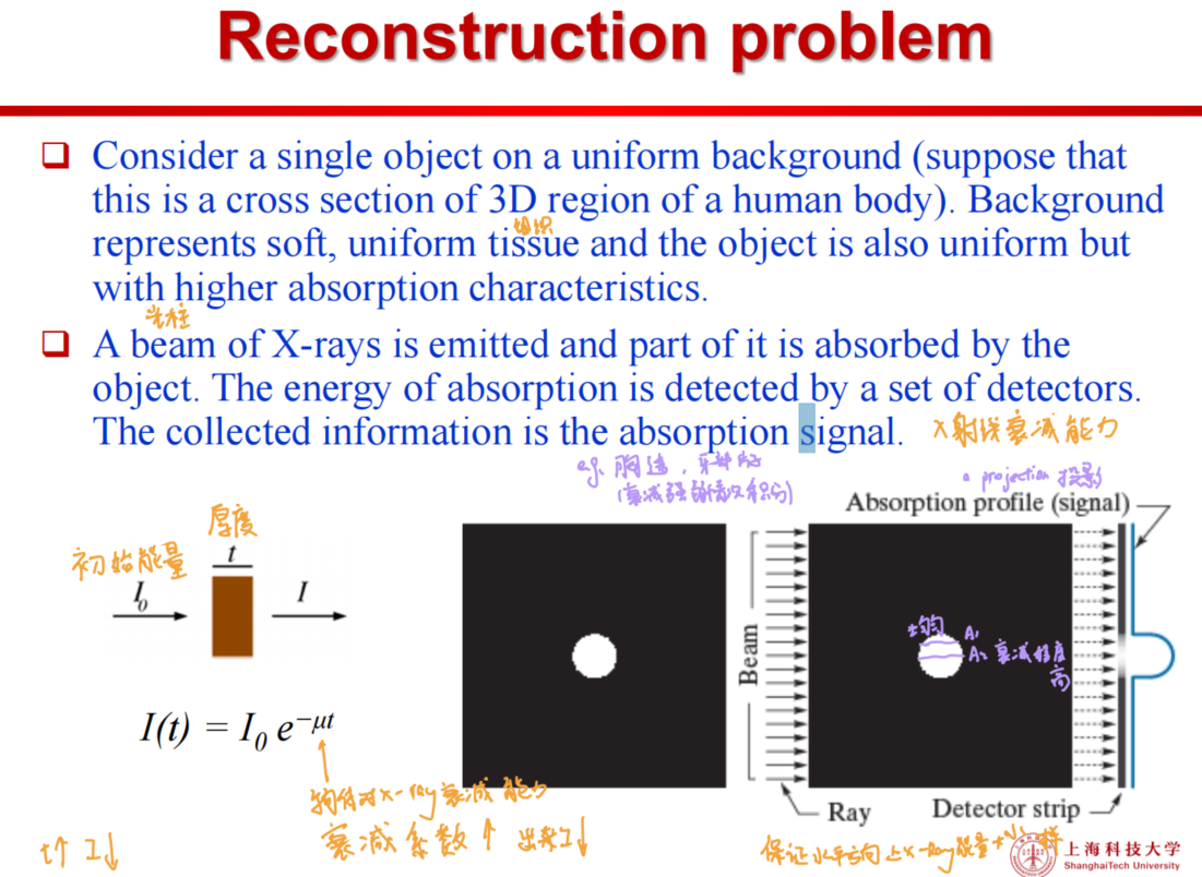
4. Image recontruction
- Recontruction problem
- Simple way: Back Projection
- 将各个方向的一维投影反向投影,投影给路径上所有点相同的信息,最终能够重建
模糊的image 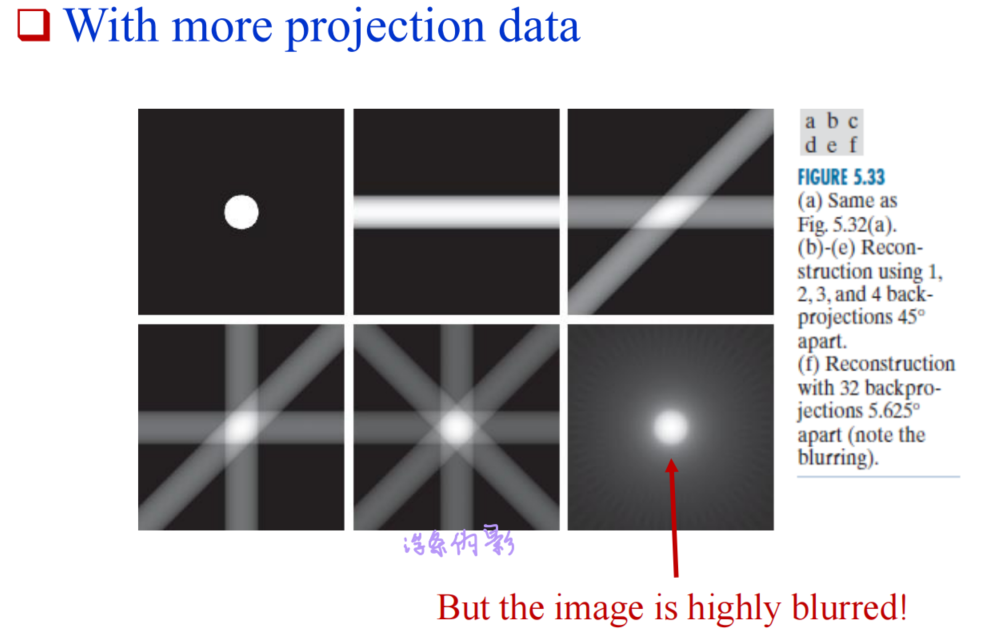
- 将各个方向的一维投影反向投影,投影给路径上所有点相同的信息,最终能够重建
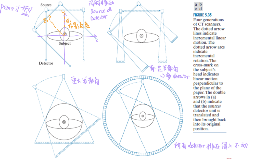
- CT
- The radon transform
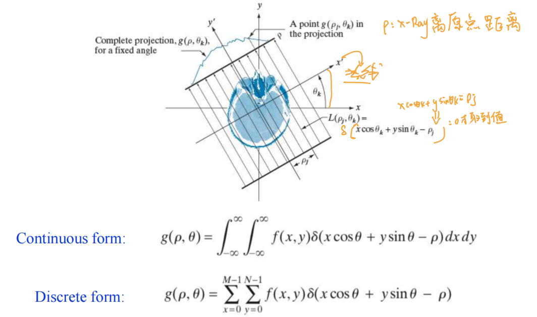
- 其中是极坐标坐标系
- Backprojection
- The Fourier-Slice Theorem
- 对projection做
1D FT就是原始图像做2D FT在该角度的切片 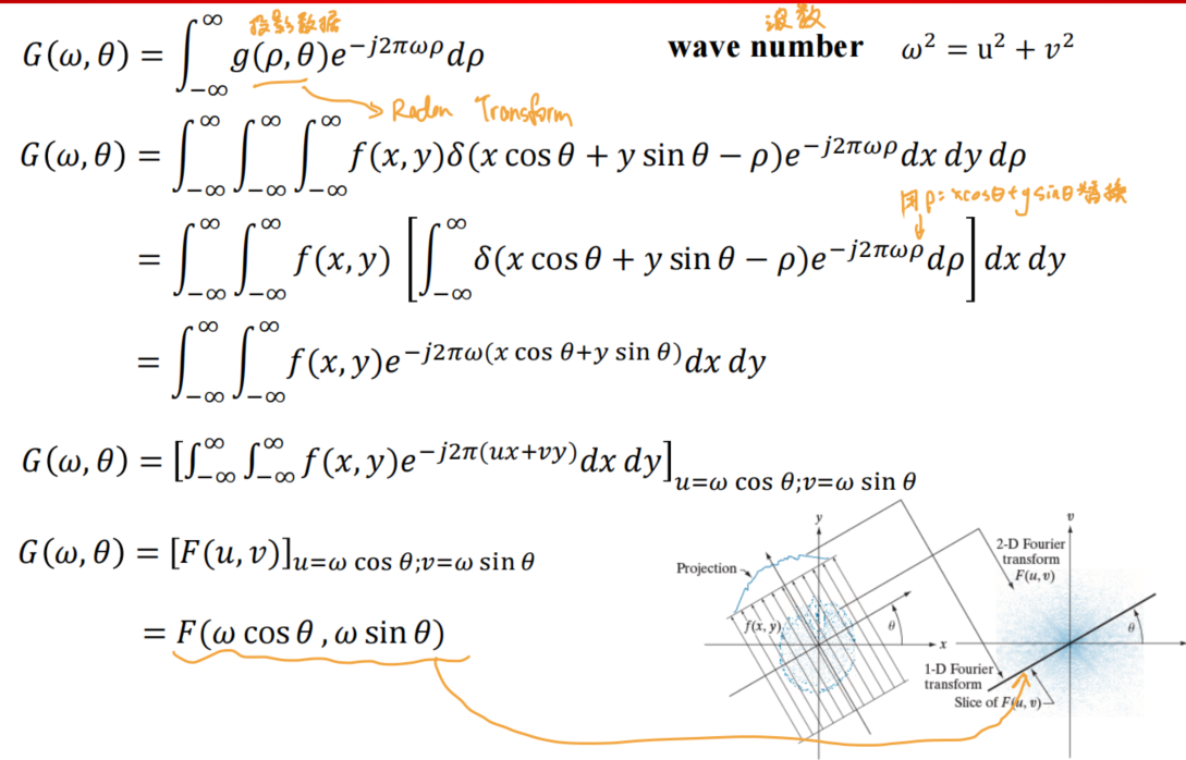
- 因此我们可以通过对每一个角度的投影进行采样,做完FT相加后,并做IDFT即可得到。但此时的均匀的采样将会导致频率域的高频成分过于稀疏,从而引入错误信息,降低重建质量
- 对projection做
- FBP (Filtered back projection)
- 引入频率域的斜坡Ramp filter
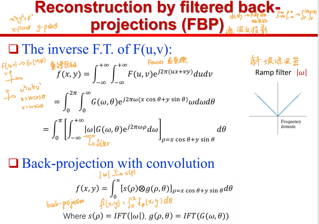
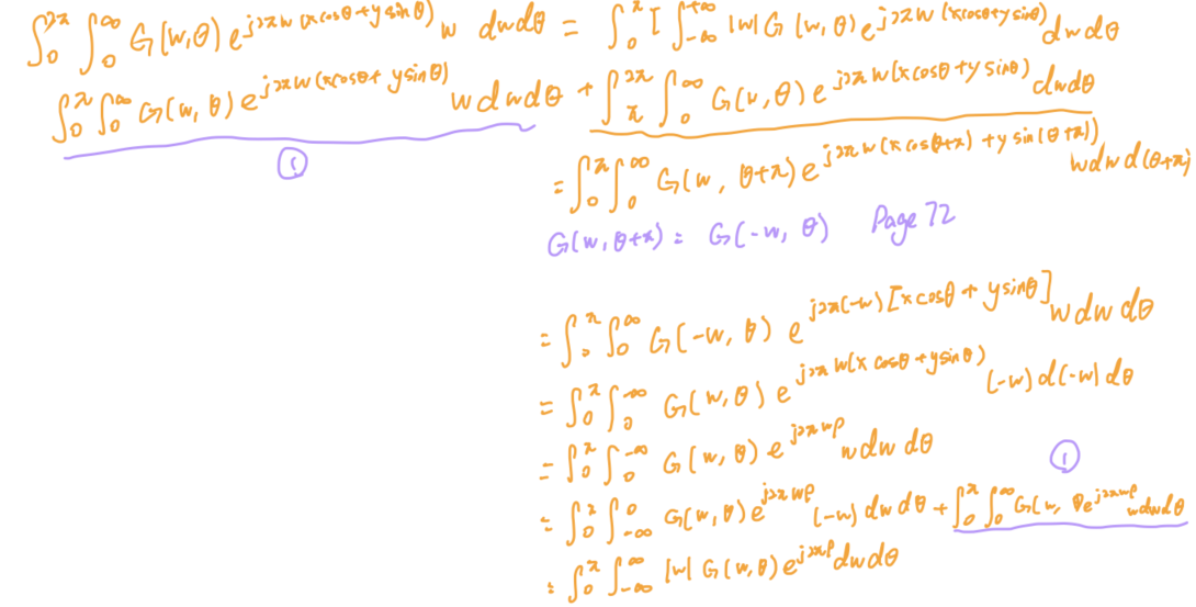
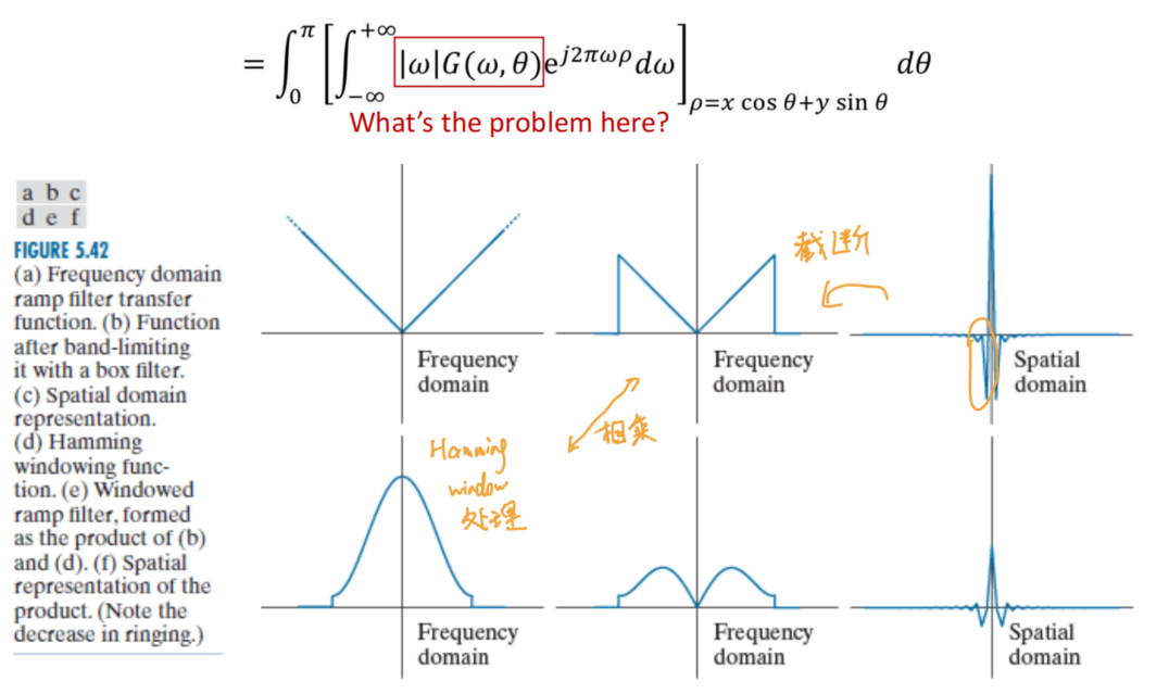
- 偏差1:
w有限带宽- Sol: bandlimit
- 偏差2: bandlimit带来的截瓣误差
- Sol: 引入hamming window,进而减少不连续程度从而减少震荡
- 最终使得光晕减少,图像更加清晰
- 偏差1:
All articles in this blog are licensed under CC BY-NC-SA 4.0 unless stating additionally.