TEULM

Related Paper

• Time Efficient Ultrasound Localization Microscopy Based on A Novel Radial Basis Function 2D Interpolation
• Increasing frame rate of echocardiography based on a novel 2D spatio-temporal meshless interpolation

Environment Building

• Matlab
• Install required toolboxs, including Communications, Bioinformatics, Image Processing, Curve Fitting, Signal Processing, Statistics and Machine Learning,Parallel Computing, and Computer Vision Toolbox.
• Run PALA_SetUpPaths.m to check whether you have successfully prepared toolboxs for your code.

How to Run ULM Code

• Step 1: Set your data read folder and data save folder path.
• Step 2: Correctly load your data and set the appropriate parameters, especially your framerate, Nbuffers, and ULM.ButterCuttofFreq.
• Step 3: Run the code.

Algorithm

• Overview: Mainly about 2D RBF interpolation method in Spatio-Temporal space
  • Radial basis fucntion
  • 2D interpolation
• Background: Because of general ULM implementation, we usually need high frame rate to get the high quality results, but in this way, it is extremely difficult in reality to get the proper data set. Therefore, introducing the 2D RBF interpolation method may improve this case by applying to the low frame rate data set, getting the results with better performance.

Pipeline Intro

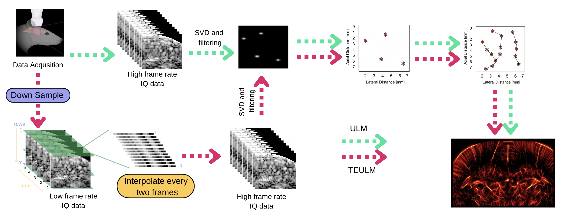
• Step 1: We need to downsample the original data set(1000 Hz) to get the low frame rate data set(100 Hz, 250 Hz, 500 Hz).
• Step 2: Apply 2D RBF interpolation to the after-downsampling data set to restore its frame rate from low one to original one.
• Step 3: Then we can run ULM code frame to get the final image result.

Algorithm Intro

• Step 1: First, downsampling data is obtained by keeping only one frame every few frames.

• Step 2: Second, we need to implement some significant functions, including:

  • 1. base_construct: To construct the base coefficient matrix by using the RBF(Euclidean distance) to get the value. Attention !!! The 2D plane need to standardlize first between $[0, 1] * [0, 1]$.
    • For base construction, you can choose random frames for constructing. For example, if your current frame rate is 100Hz, then every data file will contain 80 frames. Therefore, you had better choose all these 80 frames to construct your base matrix, so that you can interpolate more accurately. But at this time, it may lead to another problem, that is it will become much slower to construct and the matrix will become bigger.
  • 2. h_construct: To construct the new coefficient matrix by using the RBF(Euclidean distance) to get the value. Attention !!! The 2D plane need to standardlize first between $[0, 1] * [0, 1]$.
    • For h construction, the basic rule is same as the base construction. The only thing you need to focus is that you should calculate the target number of frames. Also, during this process, you can find that the relevant position of original points under the new plane scale will stay the same.
  • 3. RBF: To pre define many types of RBF functions for using, including MQ, IMQ, GA, etc.
    • Different types of RBF will have different effects. Also, they may need different shape parameter to make themselves invertible.

• Step 3: Finally, we can run the whole interpolation process to get the target result. The pseudo-code is as follows:

  # Algorithm: Applying the proposed 2D RBF interpolation method for enhancing temporal resolution
  
  # Inputs:
  # D: 3D array with dimensions M x N_c x K(original low frame number)
  # m: The bound of condition number
  # τ: Shape parameter
  
  # Outputs:
  # B: 3D array with dimensions M x N_c x Z(target high frame number)
  
  # Generating Phi, F, and X_c
  
  for ((i = 1; i <= M; i++)); do
      F = IVTS[i]  # deal with the ith row, getting the ith 2D plane
      
      Beta = Phi \ F # Get weight vector
      
      F_pre= H * beta # Interpolation
      
      B[i,:,:] = F_pre
  done

  • During this process, the only thing you need to make sure is that your Phi matrix should be invertible!!!, and then you can get the proper $\beta$ vector and finish the interpolation process. Fine-Tuning shape parameter can avoid the appearance of sigular matrix, which has a really big condition number.

Metrics Intro

1. RMSE (root mean square error)
   • A pixel level metric that depicts the similarity between the original high frame rate reconstruction image and the restored high frame rate reconstruction image by calculating their distances.
   • Formula: $RMSE = \sqrt{\sum_{i=1}^{N_{pix}}\frac{(|I_{DS} - I_1|)}{N_{pix}}}$
   • 
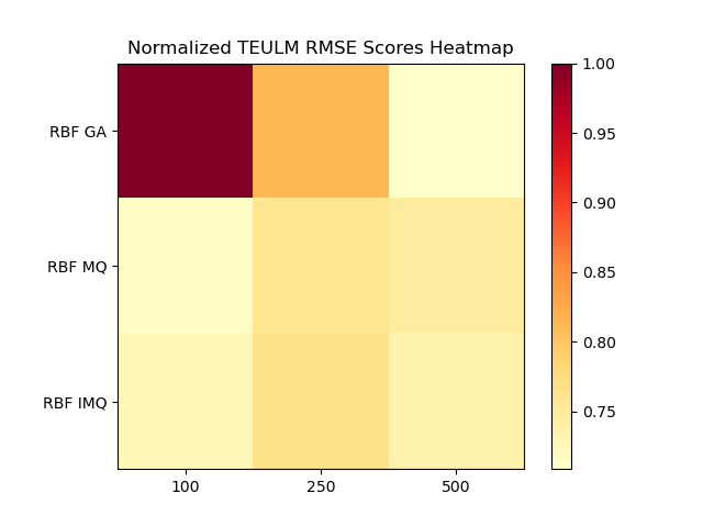
2. DICE (dice score)
   • An image level metric that depicts the similarity between the original high frame rate reconstruction image and the restored high frame rate reconstruction image by calculating their ovealapping area.
   • Formula: $DICE = \frac{2 \times |I_{DS} \cap I_1|}{|I_{DS}|\cup|I_1|}$

Advice

• For more efficient interpolation, you can implement your python code, using GPU acceleration.

For more details, you can refer to my code in github